Catastrophe vs standard loss modelling

Why is it important to understand catastrophe modelling?

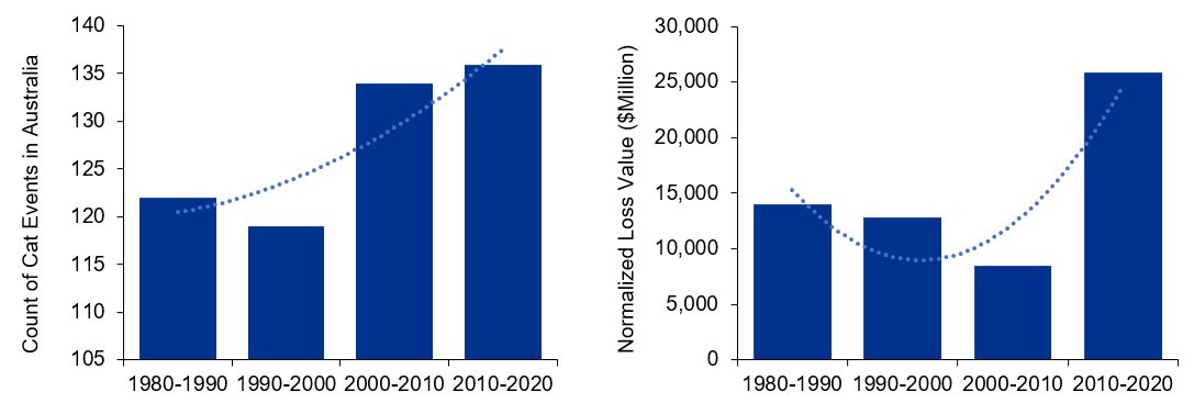
Over the past twenty years, there have been significant changes in the frequency, severity, and location of catastrophic events, which have resulted in financial losses and casualties. Some of these trends are explained through population density and urban development in new locations, but there are also trends in the underlying natural catastrophe behaviour. As an example, the figures below summarise the number of catastrophes in Australia as identified by the Insurance Council of Australia (ICA) and the normalised loss values therefrom. We can observe changes in frequency and severity, which could be the result of long weather cycles or potentially climate change.

Catastrophe modelling has been widely utilised by insurers and other relevant stakeholders to analyse and predict future losses from natural peril events. Within this context, it is useful to understand how catastrophe models work and their key differences from standard actuarial loss modelling.

Standard loss modelling

Generally, non-life insurance modelling follows a frequency-severity approach, which involves examining patterns in historical losses and fitting an algorithm to make future projections. This often involves a deterministic model, which assumes a distribution for frequency and severity. The simpler the algorithm and/or fewer explanatory variables, the greater the statistical significance of the model parameters. On the other hand, a simpler model may have lower explanatory power for volatility.

Furthermore, the standard loss model is non-geospatial in nature. That is, even where location and/or region is accounted for in the model, such as in the assessment of property value for building and contents insurance, it is used as a parameter in regression analysis. Any geographical correlation must explicitly be modelled for.

Catastrophe modelling

On the other hand, catastrophe models adopt a geospatial approach that explicitly recognises spatial and environmental factors, which impact the occurrence of catastrophic events. Such distinction is vital because the frequency, intensity, location, and shape of losses from catastrophes are largely dependent upon event parameters, such as ground motion (earthquake) and maximum three-second wind gusts (hurricane and/or cyclone). In the former case, ground motion is impacted by the nature of rocks and soil through which the energy wave passes, and for the latter, a maximum three-second wind gust depends on temperature, air pressure, centripetal acceleration, and the earth’s rotation at a specific geographical region.

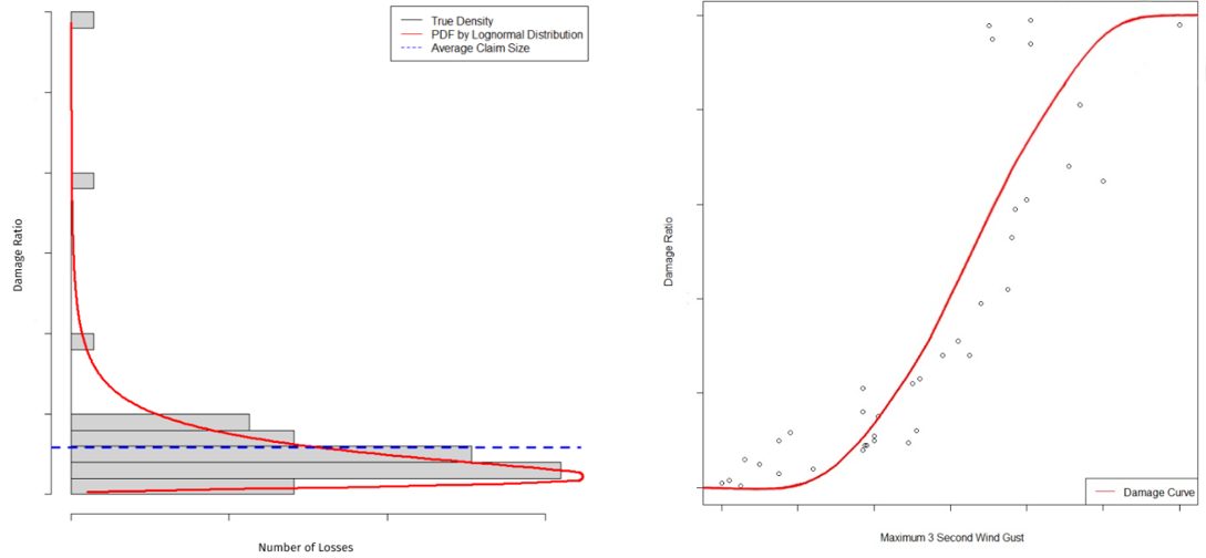
Evidently, such geospatial factors determine the intensity of the peril experienced at each location affected by the peril and inform the amount of damage to buildings, contents, and other exposures. Historical damages can be plotted against the primary characteristics of the risks that arise from the catastrophic event. For instance, peak ground acceleration (earthquake) and wind exposure (hurricane and/or cyclone). A damage curve can then be fitted to inform the associated damage for a natural peril event (right). Where the damage ratio is multiplied by the value of the assets in question, this becomes equivalent to determining an average claim size in a deterministic model (left).

However, given catastrophes are relatively infrequent events, there is a scarcity of historical data and this means that a substantial amount of professional judgment is required to fit the damage curve. In particular, catastrophe modelling focuses on the tail of the distribution, which is inevitably unstable due to the scarcity of events and the scale of impacts. Such underlying randomness and uncertainty may benefit from a stochastic approach to catastrophe modelling, whereby multiple simulations of events, areas of coverage and event metrics are obtained via stochastic catastrophe models and sampling techniques such as Monte Carlo simulation for damage.

 These simulated impacts are then summarized across cohorts of simulation years in order to determine losses at different return periods. One may have noticed that reports and similar documentation often refer to ‘1-in-100-year’ and ‘1-in-250-year’ return periods in the context of catastrophe losses. These essentially mean that there is a respective 1/100 = 1% and 1/250 = 0.4% chance of losses exceeding said impact from the peril event within any given year.

Ending note

Overall, catastrophe models are inherently different from standard actuarial models. It is envisaged that as the frequency, severity, and location of catastrophes continue to change, catastrophe models will also mature and evolve to provide more accurate and sophisticated results in modelling and predicting loss from peril events.

CPD: Actuaries Institute Members can claim two CPD points for every hour of reading articles on Actuaries Digital.