SQL and Python for IBNR Triangles

Given the rise of data science tools such as Python, R, and SQL, extensive libraries such as pandas and dplyr, and a growing emphasis on reproducible data science, there is a case for applying them more broadly to actuarial work. Here, we consider them for IBNR reserving applications. The main advantages of moving to this ‘next-generation’ approach compared to Excel are:

• Better repeatability: An automated process is easier to repeat periodically, compared to the manual data transformations in Excel at different experience investigation dates (e.g. for ingesting the most up-to-date claims data, manually inserting rows/columns and dragging down formulas).

• Better scalability: Data science tools can efficiently connect different datasets and scale to datasets of millions of rows, even on a laptop. Excel has row and column count limits, and even before this limit is reached, navigating through large Excel workbooks can be slow and difficult, especially for insurers with a sizable claims portfolio.

• Better auditability: Calculations are set out transparently in code and managed within version control systems, creating an audit trail for any changes in logic or assumptions as opposed to hardcoded cells and convoluted links.

The purpose of this article is to explore an automated approach to convert a transactional claims dataset into an IBNR triangle and calibrate Claims Development Factors (CDF) as well as the IBNR under the traditional Chain Ladder method using SQL and Python. Applying a standard chain ladder introduces the potential of code-based solutions – and opens up a wide array of improvements and extensions.

This article is an initiative of the Young Data Analytics Working Group’s Actuaries Analytical Cookbook. The code for the use case discussed in this article (‘the code’) as well as the outputs of the code is fully open-sourced and can be found here.

Dataset

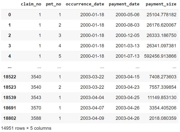
A synthetic claims dataset was used for this article, using the relatively new SynthETIC R package. This mirrors typical claims data in a tabular format, illustrated below. In particular, the dataset records occurrence date and payment date at a claim level, and caps the claims development period at 40.

The code emulates having a SQL database by using the duckdb package in Python to ingest the synthetic claims dataset. In practice, practitioners would often already have the claims data hosted on a company SQL server, so can disregard this step and run the SQL queries directly on their server. The code may require minor modification to the extent their SQL dialect used differs from duckdb’s implementation.

IBNR Triangle with SQL and Python

The example code allows for some practical issues that can arise with claims data. For example, it recognises there may not be claim records for some occurrence periods or development periods. This can be problematic if downstream processes underlying the IBNR reserving rely on the dataset having every possible occurrence and development period combination (for example, with no claims reported in the latest occurrence period due to reporting delays, the IBNR triangle generated may be incomplete).

This is easily resolved in the code with a join in SQL to another ‘dummy’ claims dataset generated with the full range of occurrence and development period combination. 

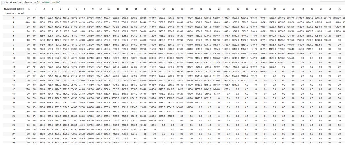
Overall, the code generates the 40 by 40 IBNR triangle with ease. A snapshot of the (cumulative) IBNR triangle is provided below.

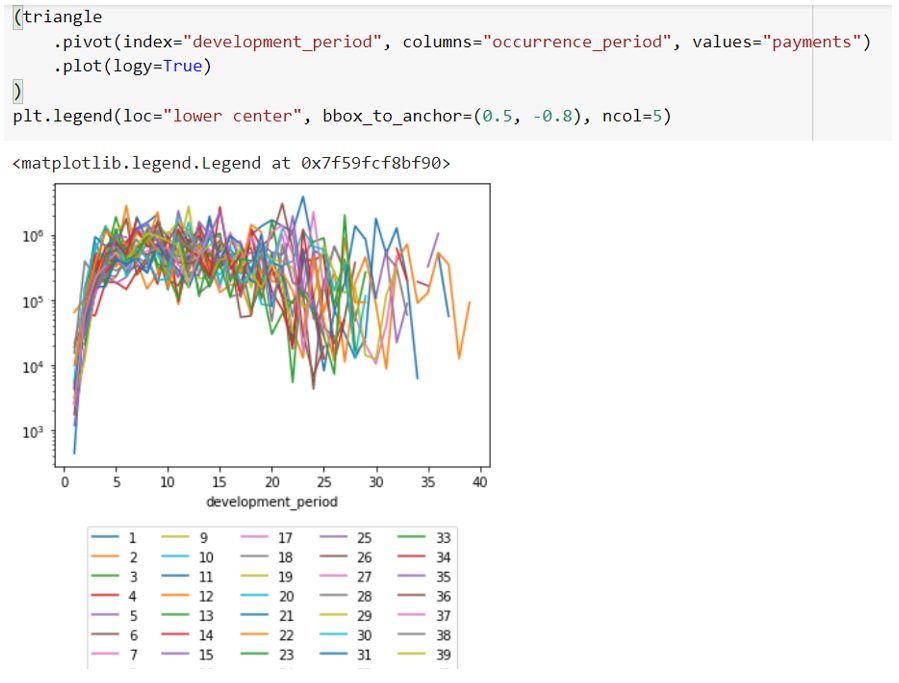
In addition, it is simple to plot the claims development by occurrence period with the pandas package in Python as shown below. This can be refined in various ways to spot trends in claims payment (e.g. claims inflation).

Projecting ultimates

Whilst the IBNR triangle in the ‘wide’ view has been generated, it may be useful to take this further and calculate the ultimate IBNR by occurrence period, claims paid/reported ratio by occurrence period, etc.

In the example, we implement a simple average-all chain ladder. The CDF is calculated with several data transformation steps using (again) the pandas package in Python. These steps include calculating cumulative claims payments, extracting the diagonal claims from the IBNR triangle as well as summing claims payment by development periods.

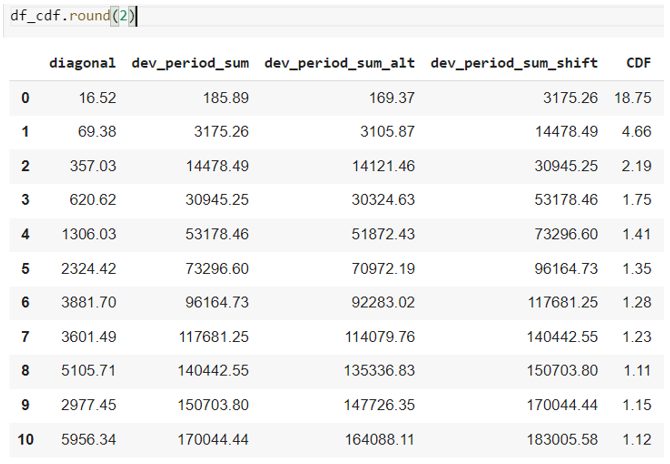
A snapshot of the output of the CDF calibrated by occurrence period is provided below^[1], from which the IBNR can be calculated as claims paid x CDF – claims paid, and the claims paid/reported ratio can be calculated as 1/CDF, for a particular occurrence period.

Other triangle methods such as the Bornhuetter-Ferguson (BF) method can be re-implemented from scratch in pandas in a similar way to how actuaries often re-implement these same triangle methods in Excel.

An alternative path is to use dedicated packages such as chainladder, which is free, open source and hosted by CAS, can also be used to produce the valuation.

Further reading

Having claims data in Python and R also allows the possibility to apply machine learning-based techniques to insurance valuation. The Machine Learning in Reserving Working Party under the IFoA has published a number of resources on this topic, usually including ready-to-run code scripts, similar to YDAWG’s Actuaries’ Analytical Cookbook.

For example, one of its publications (co-authored by one of this article’s co-authors Jacky) tests different machine learning models on a triangle. Along the way, it also explains the classic result of how fitting the lower half of the IBNR triangle with a GLM leads to the same IBNR calculated under the traditional Chain Ladder method.

CPD: Actuaries Institute Members can claim two CPD points for every hour of reading articles on Actuaries Digital.