Historical random start modelling: an alternative approach to financial projections?

Stochastic asset modelling involves the projection of financial variables for various purposes, including pension plan projections as well as financial planning. Although much of the technical debate about such modelling has been settled, a continuing issue remains how to make such modelling more accessible to laypersons. This article provides an alternative modelling approach to these projections, which relies on readily available historical data rather than bespoke internal models supported by large quantitative teams. The approach is named ‘historical random start’ (HRS) modelling for reasons explained below.

The historical random start (HRS) modelling process

HRS modelling is an approach to asset-liability modelling and scenario testing utilising historical data by:

1. selecting a sequence of financial variable(s) based on the historical behavior which fits the user’s assumptions about the relevant future (in terms of mean and standard deviation) from a larger dataset of prior historical data;
   Note: the selection of the sequence is preferably an integer number of financial cycles to ensure the full cycle length is appropriately included in the projection.

2. forming a projection of the desired periods using the selected sequence by joining the data end-on-end repeatedly; and
3. repeating this process for the desired number of simulations with the starting point of each scenario being random, hence the name ‘historical random start’.

The HRS approach is similar to, but different from bootstrapping, in that series of data are employed as simulations directly rather than utilised for parameterisation of a model which subsequently produces simulated paths for scenario testing. As Sweeting[i] explains:

“In stochastic modelling the first distinction is between bootstrapping and forward-looking approaches. For bootstrapping, all that is needed is a set of historical data for the asset classes being modelled. … The main advantage of bootstrapping is that the underlying characteristics of the data and linkages between data series are captured without having to resort to parameterisation.”

In addition to this advantage, HRS modelling also captures the historical time series autocorrelation of each financial variable. The majority of these relationships are retained under historical random start modelling apart from the points where the sequence is joined; the effect of this joining is reduced with increased length of sequence applied. This reflects the more cyclical view of investment experience provided by the HRS modelling approach compared to the traditional stochastic modelling approach.

Advantages of HRS modelling

HRS modelling has four major advantages over pure stochastic modelling, particularly where projections are required without significant resources for the development of models or distribution fitting. These advantages avoid criticisms of other stochastic models as being overly subjective and perhaps limited to the modeler’s pre-formed views or overly simple and failing to capture the “true” behavior of the relevant financial variables.

1. HRS as a concept is relatively easy to explain to laypersons – simulations are produced by direct reference to previous experience (as in the example below), rather than through the filter of a fitted stochastic model. The technique also demonstrates the importance of sequencing risk because outcome variations arise solely from different start dates.
2. HRS modeling is more visually explicit than most stochastic asset models – the user can directly see where the scenarios have come from and can easily reproduce all results. It is a fully transparent process with no requirement to fit data to a preconceived or theoretical model. It can let the data ‘speak for itself’.
3. HRS modelling directly and obviously captures all relevant elements of the selected prior experience – means, variances, skewness, kurtosis, cross correlations and auto correlations between and within individual asset classes and financial variables – by closely replicating the underlying data, apart from the points where the sequence is joined. Further, this approach can be undertaken with relatively less available information and at a much lower cost than the complex process of producing and maintaining an equivalent stochastic asset model.
4. A hallmark of HRS modelling is its flexibility, in that the sequence for repetition can be selected according to the modeler’s views as to the balance necessary between ensuring its relevance to the user’s expectations regarding future economic behavior with the need to avoid recency bias in assumption setting if desired through the use of longer periods or various other approaches such as weighting of series based on recency through discounting of older results.

Disadvantages of HRS modelling

Although HRS modelling has many significant advantages, it retains some aspects of the disadvantages of other forms of stochastic asset modelling. The three disadvantages are:

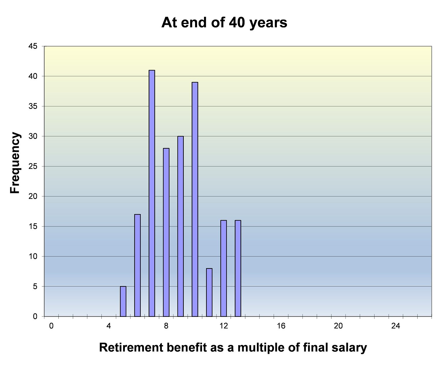
1. As with any data-driven approach, HRS modelling is limited by the availability of data, potentially to a greater extent than bootstrapping. This is because this form of modelling requires sufficient data to exceed the desired length of scenarios, in order to permit an element of randomness through the removal of some of the overall dataset from each scenario. Further, the produced simulations are unlikely to display the smooth tails of a modelled distribution, as tail events are extremely infrequent and thus the information in the tails is based on few events. This can be seen in comparing the tails of the two distributions produced by HRS modelling and stochastic asset modelling below.
2. HRS modelling’s application in projections is only suitable where asset class returns are employed in ‘real’ terms relative to either the price or salary inflation existing at the time of the returns. This is because underlying economic conditions have the effect of inflating asset class behaviour such that this information is only comparable once this influence is offset. However, this issue is not a significant disadvantage for two reasons.
   a. It is simple to address this limitation simply by deflating historical returns by prevailing inflation to ensure that historical data is comparable across the desired dataset.
   b. This limitation is irrelevant in the context of replacement rate-based retirement income projection because such analyses provide insight into retirement outcomes within the context of existing economic conditions rather than in potentially misleading nominal terms.

3. HRS modelling’s approach is extremely vulnerable to misapplication through a poor choice of sequence start or end point. Because the approach is quite accessible, there is a danger of misunderstanding the importance of these choices, which could lead to discontinuous scenarios or choice of a period focusing solely upon one desired assumption (e.g. the mean) without consideration of other relevant assumptions (e.g. standard deviations and correlations/autocorrelations). The modeler must be careful to ensure such misapplication does not occur.

HRS in practice

To demonstrate the historical random start process, an example of HRS modelling is compared to stochastic modelling utilising the Austmod stochastic asset model,[ii] which is capable of producing both stochastic asset modelling and HRS modelling.

The example involves a 40-year projection of the retirement balance of an Australian individual with four years of past plan membership and retiring in 40 years’ time. The retirement balance is expressed as a multiple of final salary assuming the member invested in a “balanced” portfolio throughout their career. The historical random start modelling process in this instance utilises a 44-year sequence ending 31 December 2017 with 200 historical random start simulations. This results in the following average results for the shares, bonds, wage inflation and price inflation financial variables as well as for the balanced investment portfolio:

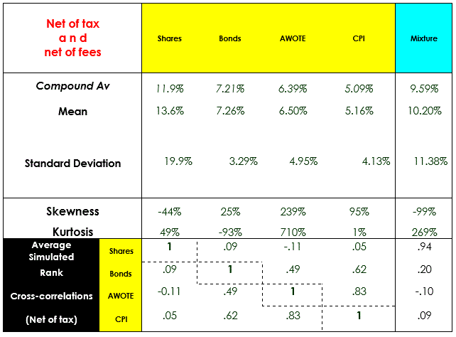
The distribution of outcomes for the retiree’s retirement balance as a multiple of final salary can be seen below.

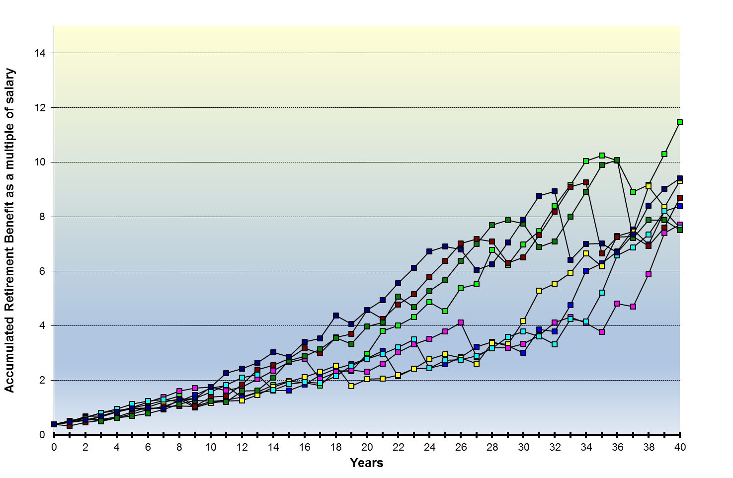
A ‘snail trail’ of the first eight scenarios is also shown to indicate how the calculated benefit multiple might rise and fall from year to year.

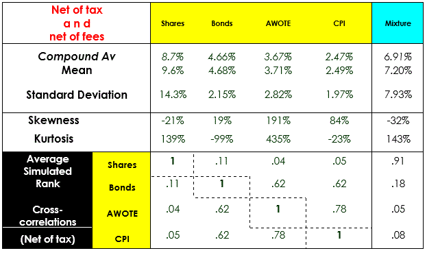
By contrast, stochastic asset modelling output is provided below for the same simulation exercise. This output is derived from application of the Austmod stochastic asset model which projects financial variable behaviour as a set[iii] of auto-correlated and rank cross-correlated normal distributions which are then transformed to reflect assumed standard skewness and kurtosis. The statistical output for the shares, bonds, wage inflation and price inflation variables and the balanced portfolio are again provided below:

As for the HRS modelling, the distribution of 40-year retirement balance outcomes is provided below together with a ‘snail trail’ of the first eight scenarios:

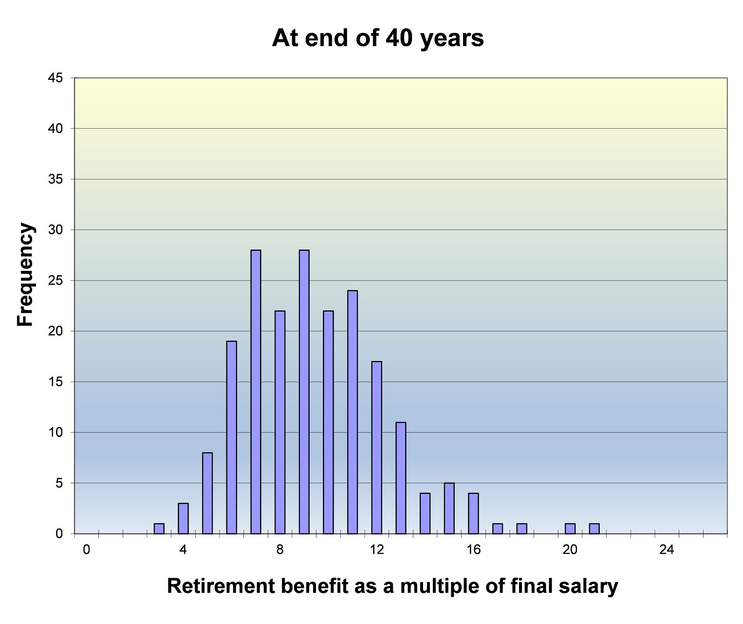
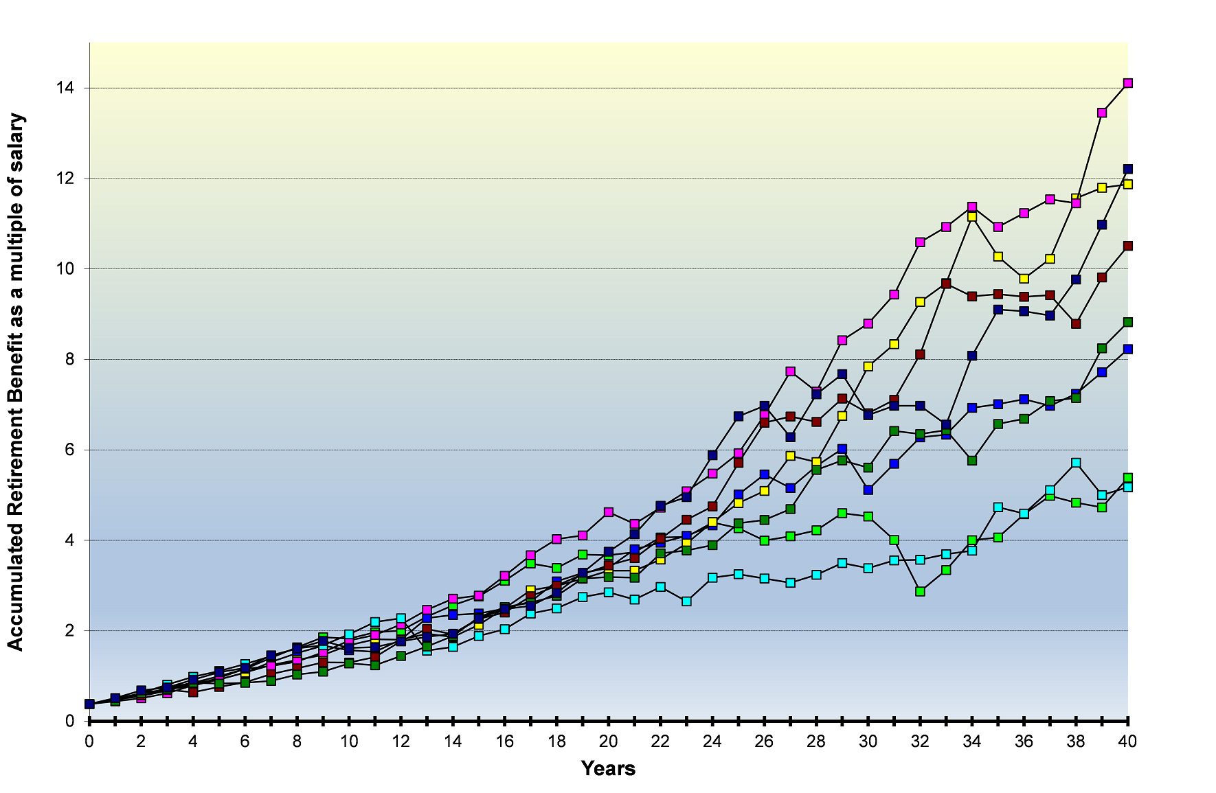
It can be seen from a comparison of the HRS modelling and Austmod stochastic modelling that the results are quite similar in terms of correlations and the Sharpe ratios (mean divided by standard deviation) of the displayed financial variables. The means are slightly different due to the HRS sequences reflecting the chosen historical period whereas the stochastic model output means are primarily determined by the setting of most Austmod assumptions being based on a continuation of economic conditions for two years from the endpoint of the underlying dataset and a long-term average price inflation of 2.5%pa. However, because this example is based on multiples of salary (or had it been based on wage-adjusted discounted values) the projection results are not misleading.

Overall, it is obvious from this output that despite its lower technical rigour and attendant reduced need for modelling knowledge, the HRS modelling approach provides fairly similar results to an established stochastic asset model whilst retaining the advantageous qualities of ease of explanation and transparency of approach.

Conclusion

The historical random start modelling approach can often be considered a valid alternative to stochastic asset modelling – for example when it is challenging to develop internal estimates of future market performance or where technical resources for model development are limited.  HRS modelling can serve as a sensitivity/stress test compared to existing models. Its output is more easily explainable and understood since it merely replicates past economic behaviour.

However, this approach should be approached with suitable understanding of its limitations, in that it is data intensive (requiring a dataset preferably in excess of the projection period desired) and like all modelling approaches is subject to misapplication risk.  Also, the period chosen from which the data is drawn may not be reflective of the future. For these reasons, such modelling is more suitable in the context of fairly simple projections or where technical knowledge or resources are limited. As long as the user bears in mind these caveats in employing the method, historical random start modelling can be a valuable tool in making the process of performing financial projections much easier.

CPD: Actuaries Institute Members can claim two CPD points for every hour of reading articles on Actuaries Digital.